b1field#
- mrtwin.b1field(shape, nmodes=1, b1range=(0.5, 2.0), shift=None, dphi=0.0, coil_width=1.1, ncoils=2, nrings=None, mask=None, cache=None, cache_dir=None)[source]#
Simulate inhomogeneous B1+ fields.
Adapted from SigPy [1].
- Parameters:
shape (Sequence[int]) – Size of the matrix
(ny, nx)(2D) or(nz, ny, nx)(3D) for the B1+ field.nmodes (int, optional) – Number of B1+ modes. First mode is
CPmode, second isgradientmode, and so on. The default is1.b1range (Sequence[float], optional) – Range of B1+ magnitude. The default is
(0.5, 2.0).shift (Sequence[int], optional) – Displacement of the coil center with respect to matrix center. The default is
(0, 0)/(0, 0, 0).dphi (float, optional) – Bulk coil angle in
[deg]. The default is0.0°.coil_width (float, optional) – Width of the coil, with respect to image dimension. The default is
1.1.ncoils (int, optional) – Number of transmit coil elements. Standard coils have
2channels operating in quadrature. To support multiple modes (e.g., PTX), increase this number. The default is4.nrings (int, optional) – Number of rings for a cylindrical hardware set-up. The default is
ncoils // 4.mask (np.ndarray | None, optional) – Region of support of the object of shape
(ny, nx)(2D) or(nz, ny, nx)(3D). The default isNone.cache (bool | None, optional) – If
True, cache the phantom. The default isTruefor 3D phantoms andFalsefor single-slice 2D.cache_dir (CacheDirType, optional) – cache_directory for phantom caching. The default is
None(~/.cache/mrtwin).
- Returns:
smap – Complex spatially varying b1+ maps of shape
(nmodes, ny, nx)(2D) or(nmodes, nz, ny, nx)(3D). Magnitude of the map represents the relative flip angle scaling (wrt to the nominal).- Return type:
np.ndarray
Example
>>> from mrtwin import b1field
We can generate a 2D B1+ field map of shape
(ny=128, nx=128)by:>>> b1map = b1field((128, 128))
Field center and rotation can be modified by
shiftanddphiarguments:>>> b1map = b1field((128, 128), shift=(-3, 5), dphi=30.0) # center shifted by (dy, dx) = (-3, 5) pixels and rotated by 30.0 degrees.
B1+ values range and steepness of variation can be specified using
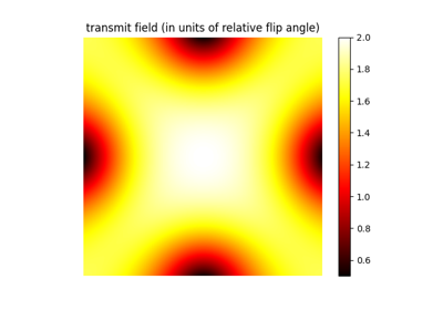
b1rangeandcoil_widtharguments:>>> # transmit coil is 4 times bigger than FOV (e.g., body coil) and >>> # B1+ scalings are between (0.8, 1.2) the nominal flip angle (e.g., 3T scanner) >>> b1map3T = b1field((128, 128), b1range=(0.8, 1.2), coil_width=4.0) >>> >>> # transmit coil is 1.1 times bigger than FOV (e.g., head coil) and >>> # B1+ scalings are between (0.5, 2.0) the nominal flip angle (e.g., 7T scanner) >>> b1map7T = b1field((128, 128), b1range=(0.5, 2.0), coil_width=1.1)
Multiple orthogonal modes can be simulated by
nmodesargument. For example, CP mode and gradient mode can be obtained as:>>> b1map = b1field((128, 128), nmodes=2) # b1map[0] is CP, b1map[1] is gradient mode.
Three dimensional B1+ maps of shape
(nz, ny, nx)can be obtained as:>>> b1map = b1field((128, 128, 128))
Beware that this will require more memory.
References
[1] mikgroup/sigpy
