Shepp-Logan Phantom

Example of Shepp-Logan phantom creation.

This examples show how to generate numerical phantoms based on the Shepp-Logan model.

import matplotlib.pyplot as plt
import numpy as np

from mrtwin import shepplogan_phantom

Basic Usage

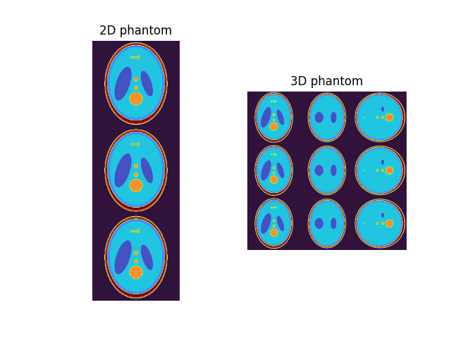
A digital Shepp-Logan phantom can be created as:

phantom2D = shepplogan_phantom(ndim=2, shape=200)  # 2D phantom
phantom3D = shepplogan_phantom(ndim=3, shape=200)  # 3D phantom

where shape is a matrix size, which can be provided as a scalar (isotropic matrix) or a ndim-length tuple.

The phantoms here created are sparse, i.e., they consists of an integer (*spatial_shape) shaped np.ndarray whose values represent the label (i.e., the index) identifying each tissue type (e.g., Gray Matter, White Matter, CSF) and a list of (nclasses,) dictionaries each containing the (M0, T1, T2, T2*, Chi) values for each class:

example2D = np.concatenate((phantom2D, phantom2D, phantom2D), axis=0)

example3Dax = np.concatenate((phantom3D[100], phantom3D[100], phantom3D[100]), axis=0)
example3Dcor = np.concatenate(
    (phantom3D[::-1, 100], phantom3D[::-1, 100], phantom3D[::-1, 100]), axis=0
)
example3Dsag = np.concatenate(
    (
        phantom3D[::-1, :, 100],
        phantom3D[::-1, :, 100],
        phantom3D[::-1, :, 100],
    ),
    axis=0,
)
example3D = np.concatenate((example3Dax, example3Dcor, example3Dsag), axis=1)

fig1, ax1 = plt.subplots(1, 2)
ax1[0].imshow(example2D, cmap="turbo"), ax1[0].axis("off"), ax1[0].set_title(
    "2D phantom"
)
ax1[1].imshow(example3D, cmap="turbo"), ax1[1].axis("off"), ax1[1].set_title(
    "3D phantom"
)
plt.show()

The (M0, T1, T2, T2*, Chi) properties can be direcly accessed as:

_, _ = print("M0:", end="\t"), print(phantom2D.M0)  # same for phantom3D
_, _ = print("T1 (ms):", end="\t"), print(phantom2D.T1)
_, _ = print("T2 (ms):", end="\t"), print(phantom2D.T2)
_, _ = print("T2* (ms):", end="\t"), print(phantom2D.T2s)
_, _ = print("Chi:", end="\t"), print(phantom2D.Chi)

M0:     [0.   1.   0.86 0.77 1.   1.   1.   1.   1.   1.   1.   1.  ]
T1 (ms):        [   0.      4200.       998.1393   680.66815  342.50705 1050.
 1050.       350.      1549.5471   342.50705  700.       552.36127]
T2 (ms):        [   0. 1990.  100.   80.   70.   50.   50.   15.  200.   70.  150.   50.]
T2* (ms):       [  0.       243.06877   73.46702   62.067276  64.09466   42.323383
  42.323383  14.274805 116.12312   64.09466   97.293144  46.912655]
Chi:    [ 4.00e-07 -9.00e-06 -9.00e-06 -9.00e-06  3.28e-06 -9.04e-06 -9.04e-06
 -8.44e-06 -9.00e-06  3.28e-06 -9.00e-06  3.28e-06]

If required, the properties dictionary can be directly accessed as:

print(phantom2D.properties)

{'M0': array([0.  , 1.  , 0.86, 0.77, 1.  , 1.  , 1.  , 1.  , 1.  , 1.  , 1.  ,
       1.  ], dtype=float32), 'T1': array([   0.     , 4200.     ,  998.1393 ,  680.66815,  342.50705,
       1050.     , 1050.     ,  350.     , 1549.5471 ,  342.50705,
        700.     ,  552.36127], dtype=float32), 'T2': array([   0., 1990.,  100.,   80.,   70.,   50.,   50.,   15.,  200.,
         70.,  150.,   50.], dtype=float32), 'T2s': array([  0.      , 243.06877 ,  73.46702 ,  62.067276,  64.09466 ,
        42.323383,  42.323383,  14.274805, 116.12312 ,  64.09466 ,
        97.293144,  46.912655], dtype=float32), 'Chi': array([ 4.00e-07, -9.00e-06, -9.00e-06, -9.00e-06,  3.28e-06, -9.04e-06,
       -9.04e-06, -8.44e-06, -9.00e-06,  3.28e-06, -9.00e-06,  3.28e-06],
      dtype=float32)}

e.g., to be passed as **kwargs to a simulator routine.

Notice that segmentation can be accessed directly (in read-only mode) via square bracked indexing, similarly to numpy arrays.

A basic summary of the properties can be accessed via the __repr__ attribute (i.e., enabling pretty printing):

print(phantom2D)
print(phantom3D)

Crisp Shepp-Logan phantom with following properties:
Number of spatial dimensions: 2
Tissue properties: dict_keys(['M0', 'T1', 'T2', 'T2s', 'Chi'])
Matrix size: (200, 200)

Crisp Shepp-Logan phantom with following properties:
Number of spatial dimensions: 3
Tissue properties: dict_keys(['M0', 'T1', 'T2', 'T2s', 'Chi'])
Matrix size: (200, 200, 200)

We can obtain a “dense” phantom, i.e., an object without segmentation whose (M0, T1, T2, T2*, Chi) properties are stored as parametric maps rather than the individual values of each tissue class as:

phantom2D = phantom2D.as_numeric()

# Print summary

print(phantom2D)

# Display parameter maps

fig3, ax3 = plt.subplots(1, 5)

im0 = ax3[0].imshow(phantom2D.M0, cmap="gray")
ax3[0].axis("off"), ax3[0].set_title("M0 [a.u.]")
fig3.colorbar(im0, ax=ax3[0], fraction=0.046, pad=0.04)

im1 = ax3[1].imshow(phantom2D.T1, cmap="magma")
ax3[1].axis("off"), ax3[1].set_title("T1 [ms]")
fig3.colorbar(im1, ax=ax3[1], fraction=0.046, pad=0.04)

im2 = ax3[2].imshow(phantom2D.T2, cmap="viridis", vmax=150)
ax3[2].axis("off"), ax3[2].set_title("T2 [ms]")
fig3.colorbar(im2, ax=ax3[2], fraction=0.046, pad=0.04)

im3 = ax3[3].imshow(phantom2D.T2s, cmap="viridis", vmax=150)
ax3[3].axis("off"), ax3[3].set_title("T2* [ms]")
fig3.colorbar(im3, ax=ax3[3], fraction=0.046, pad=0.04)

im4 = ax3[4].imshow(phantom2D.Chi, cmap="gray")
ax3[4].axis("off"), ax3[4].set_title("Chi")
fig3.colorbar(im4, ax=ax3[4], fraction=0.046, pad=0.04)

plt.tight_layout()
plt.show()

Crisp Shepp-Logan phantom with following properties:
Number of spatial dimensions: 2
Tissue properties: dict_keys(['M0', 'T1', 'T2', 'T2s', 'Chi'])
Matrix size: (200, 200)

Dense phantom can be also directly generated as:

phantom2D = shepplogan_phantom(
    ndim=2, shape=200, segtype=False
)  # default is segtype="crisp"

# Print summary

print(phantom2D)

Crisp Shepp-Logan phantom with following properties:
Number of spatial dimensions: 2
Tissue properties: dict_keys(['M0', 'T1', 'T2', 'T2s', 'Chi'])
Matrix size: (200, 200)

Hereafter, without loss of generality, we will use 2D phantoms.

The physical parameter of each tissue class are calculated by default for a field strength of 1.5 T.

This can be changed via the B0 argument:

# B0 strengths
B0 = [0.55, 1.5, 3.0, 7.0, 11.7, 13.3]  # field strengths in [T]

# Generate phantoms with different field strengths
phantomB0 = [
    shepplogan_phantom(ndim=2, shape=200, B0=strength, segtype=False) for strength in B0
]

# Display
T1 = np.concatenate([phantom.T1 for phantom in phantomB0], axis=1)
T2 = np.concatenate([phantom.T2 for phantom in phantomB0], axis=1)
T2s = np.concatenate([phantom.T2s for phantom in phantomB0], axis=1)

fig5, ax5 = plt.subplots(3, 1)

im1 = ax5[0].imshow(T1, cmap="magma", vmax=5000)
ax5[0].axis("off"), ax5[0].set_title("T1 [ms]")
fig5.colorbar(im1, ax=ax5[0], fraction=0.046, pad=0.04)

im2 = ax5[1].imshow(T2, cmap="viridis", vmax=150)
ax5[1].axis("off"), ax5[1].set_title("T2 [ms]")
fig5.colorbar(im2, ax=ax5[1], fraction=0.046, pad=0.04)

im3 = ax5[2].imshow(T2s, cmap="viridis", vmax=100)
ax5[2].axis("off"), ax5[2].set_title("T2* [ms]")
fig5.colorbar(im3, ax=ax5[2], fraction=0.046, pad=0.04)

plt.tight_layout()
plt.show()

In addition to single pool model, we provide 3 multi-pool models:

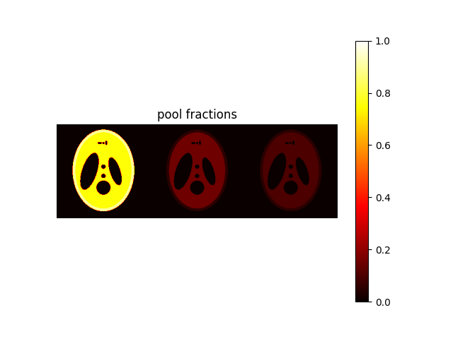
1. "mw-model": a two-pool model where free water is divided in two compartments, i.e., intra-/extra-cellular water (long T1 / T2) and myelin water (short T1 / T2). The model include chemical exchange between the two pools. Parameters are (MWF, T1, T2, k, chemshift).

2. "mt-model": a two-pool model consisting in free water and bound water. Free water includes both intra-/extra-cellular and myelin water (as in the single-pool model), while bound water corresponds to a macromolecular pool with the same T1 as the free water and no T2 (i.e., no transverse magnetization). The model include magnetization transfer between the two pools. Parameters are (MVF, T1, T2, k).

3. "mwmt-model": a three-pool model consisting in intra-/extra-cellular water, myelin water and bound water. The model include chemical exchange between the two free water pools and magnetizion transfer between myelin water and bound water. Parameters are (MWF, MVF, T1, T2, k).

Here we will display the latter, as it represents the most general case.

# model="single-pool" is the default, while "mw-model" and "mt-model" corresponds to cases 1. and 2.
phantom_multi = shepplogan_phantom(ndim=2, shape=200, model="mwmt-model", segtype=False)

MWF corresponds to the myelin water fraction, while MVF to the bound water fraction. We assume that intra-extracellular water fraction = 1 - (MWF + MVF):

MWF = phantom_multi.MWF
MVF = phantom_multi.MVF
IEWF = (1 - (MWF + MVF)) * (MWF > 0)
weight = np.concatenate((IEWF, MWF, MVF), axis=1)

plt.figure()
plt.imshow(weight, vmin=0, vmax=1, cmap="hot"), plt.axis("off"), plt.title(
    "pool fractions"
), plt.colorbar()
plt.show()

T1 and T2 for the two free water pools are stacked along the first axis, with n=0 being the intra-/extra-cellular water (long T1 / T2) and n=1 being the myelin water (short T1 / T2):

T1 = np.concatenate((phantom_multi.T1[0], phantom_multi.T1[1]), axis=1)
T2 = np.concatenate((phantom_multi.T2[0], phantom_multi.T2[1]), axis=1)

fig6, ax6 = plt.subplots(2, 1)

im1 = ax6[0].imshow(T1, cmap="magma", vmax=1500)
ax6[0].axis("off"), ax6[0].set_title("T1 [ms]")
fig6.colorbar(im1, ax=ax6[0], fraction=0.046, pad=0.04)

im2 = ax6[1].imshow(T2, cmap="viridis", vmax=150)
ax6[1].axis("off"), ax6[1].set_title("T2 [ms]")
fig6.colorbar(im2, ax=ax6[1], fraction=0.046, pad=0.04)

<matplotlib.colorbar.Colorbar object at 0x7f3dc1245d20>

k represent the non-directional exchange rates in [Hz], with n=0 being the chemical exchange rate between the two free water pools and n=1 being magnetization transfer rate between the myelin and bound water:

k = np.concatenate((phantom_multi.k[0], phantom_multi.k[1]), axis=1)

plt.figure()
plt.imshow(k, cmap="hot"), plt.axis("off"), plt.title(
    "exchange rate [Hz]"
), plt.colorbar()
plt.show()

Similarly to the single pool model, mrtwin also supports a sparse (segtype="crisp") representation.

Caching mechanism

To reduce loading times, mrtwin implements a caching mechanism.

If cache argument is set to True (default behaviour for ndim=3), each phantom segmentation (identified by the number of spatial dimensions, tissue model, segmentation type and matrix shape) is saved on the disk in npy format.

The path is selected according to the following hierachy (inspired by brainweb-dl):

1. User-specific argument (cache_dir)

2. MRTWIN_DIR environment variable

3. ~/.cache/mrtwin folder