Brainweb Phantom

Example of Brainweb phantom creation.

This examples show how to generate numerical phantoms based on the Brainweb dataset.

import matplotlib.pyplot as plt
import numpy as np

from mrtwin import brainweb_phantom

Basic Usage

The Brainweb database consists of a set of 20 normal brains (ids equal to [4, 5, 6, 18, 20, 38, 41-54]) at a nominal 0.5 mm isotropic resolution and a shape of (nz, ny, nx) = (362, 434, 362).

A digital Brainweb phantom can be created as:

phantom2D = brainweb_phantom(ndim=2, subject=4, segtype="fuzzy")  # 2D phantom
phantom3D = brainweb_phantom(ndim=3, subject=4, segtype="fuzzy")  # 3D phantom

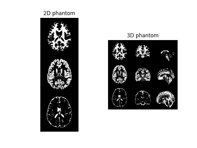
The phantoms here created are sparse, i.e., they consists of a (nclasses, *spatial_shape) shaped np.ndarray representing the probabilistic maps of each tissue type (e.g., Gray Matter, White Matter, CSF) and a list of (nclasses,) dictionaries each containing the (M0, T1, T2, T2*, Chi) values for each class:

example2D = np.concatenate((phantom2D[3], phantom2D[2], phantom2D[1]), axis=0)

example3Dax = np.concatenate(
    (phantom3D[3, 100], phantom3D[2, 100], phantom3D[1, 100]), axis=0
)
example3Dcor = np.concatenate(
    (phantom3D[3, ::-1, 100], phantom3D[2, ::-1, 100], phantom3D[1, ::-1, 100]), axis=0
)
example3Dsag = np.concatenate(
    (
        phantom3D[3, ::-1, :, 100],
        phantom3D[2, ::-1, :, 100],
        phantom3D[1, ::-1, :, 100],
    ),
    axis=0,
)
example3D = np.concatenate((example3Dax, example3Dcor, example3Dsag), axis=1)

fig1, ax1 = plt.subplots(1, 2)
ax1[0].imshow(example2D, cmap="gray"), ax1[0].axis("off"), ax1[0].set_title(
    "2D phantom"
)
ax1[1].imshow(example3D, cmap="gray"), ax1[1].axis("off"), ax1[1].set_title(
    "3D phantom"
)
plt.show()

The (M0, T1, T2, T2*, Chi) properties can be direcly accessed as:

_, _ = print("M0:", end="\t"), print(phantom2D.M0)  # same for phantom3D
_, _ = print("T1 (ms):", end="\t"), print(phantom2D.T1)
_, _ = print("T2 (ms):", end="\t"), print(phantom2D.T2)
_, _ = print("T2* (ms):", end="\t"), print(phantom2D.T2s)
_, _ = print("Chi:", end="\t"), print(phantom2D.Chi)

M0:     [0.   1.   0.86 0.77 1.   1.   1.   1.   1.   1.   1.   1.  ]
T1 (ms):        [   0.      4200.       998.1393   680.66815  342.50705 1050.
 1050.       350.      1549.5471   342.50705  700.       552.36127]
T2 (ms):        [   0. 1990.  100.   80.   70.   50.   50.   15.  200.   70.  150.   50.]
T2* (ms):       [  0.       243.06877   73.46702   62.067276  64.09466   42.323383
  42.323383  14.274805 116.12312   64.09466   97.293144  46.912655]
Chi:    [ 4.00e-07 -9.00e-06 -9.00e-06 -9.00e-06  3.28e-06 -9.04e-06 -9.04e-06
 -8.44e-06 -9.00e-06  3.28e-06 -9.00e-06  3.28e-06]

If required, the properties dictionary can be directly accessed as:

print(phantom2D.properties)

{'M0': array([0.  , 1.  , 0.86, 0.77, 1.  , 1.  , 1.  , 1.  , 1.  , 1.  , 1.  ,
       1.  ], dtype=float32), 'T1': array([   0.     , 4200.     ,  998.1393 ,  680.66815,  342.50705,
       1050.     , 1050.     ,  350.     , 1549.5471 ,  342.50705,
        700.     ,  552.36127], dtype=float32), 'T2': array([   0., 1990.,  100.,   80.,   70.,   50.,   50.,   15.,  200.,
         70.,  150.,   50.], dtype=float32), 'T2s': array([  0.      , 243.06877 ,  73.46702 ,  62.067276,  64.09466 ,
        42.323383,  42.323383,  14.274805, 116.12312 ,  64.09466 ,
        97.293144,  46.912655], dtype=float32), 'Chi': array([ 4.00e-07, -9.00e-06, -9.00e-06, -9.00e-06,  3.28e-06, -9.04e-06,
       -9.04e-06, -8.44e-06, -9.00e-06,  3.28e-06, -9.00e-06,  3.28e-06],
      dtype=float32)}

e.g., to be passed as **kwargs to a simulator routine.

Notice that segmentation can be accessed directly (in read-only mode) via square bracked indexing, similarly to numpy arrays.

A basic summary of the properties can be accessed via the __repr__ attribute (i.e., enabling pretty printing):

print(phantom2D)
print(phantom3D)

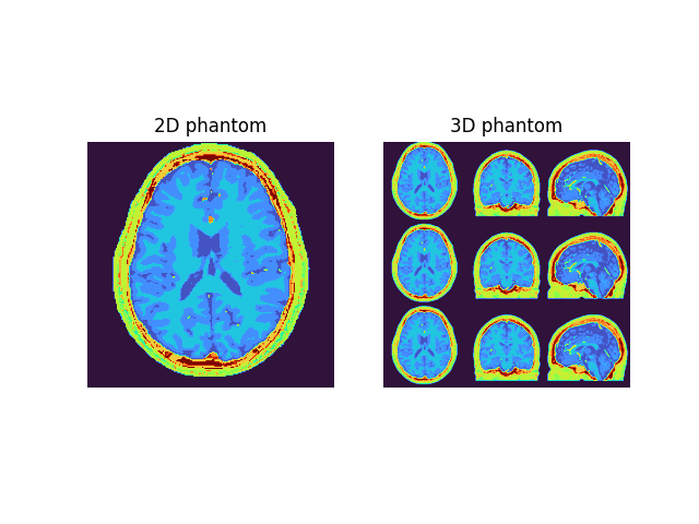
# We also provide a crisp segmentation, which has a lower memory footprint
# at cost of a coarser approximation (i.e., a piecewise-constant tissue model)-
#
# This can be obtained starting from the `"fuzzy"` phantom as:

phantom2D = phantom2D.as_crisp()
phantom3D = phantom3D.as_crisp()

# Print summary

print(phantom2D)
print(phantom3D)

# Display spatial segmentations

example2D = phantom2D

example3Dax = np.concatenate((phantom3D[100], phantom3D[100], phantom3D[100]), axis=0)
example3Dcor = np.concatenate(
    (phantom3D[::-1, 100], phantom3D[::-1, 100], phantom3D[::-1, 100]), axis=0
)
example3Dsag = np.concatenate(
    (phantom3D[::-1, :, 100], phantom3D[::-1, :, 100], phantom3D[::-1, :, 100]), axis=0
)
example3D = np.concatenate((example3Dax, example3Dcor, example3Dsag), axis=1)

fig2, ax2 = plt.subplots(1, 2)
ax2[0].imshow(example2D, cmap="turbo"), ax2[0].axis("off"), ax2[0].set_title(
    "2D phantom"
)
ax2[1].imshow(example3D, cmap="turbo"), ax2[1].axis("off"), ax2[1].set_title(
    "3D phantom"
)
plt.show()

Fuzzy Brainweb phantom with following properties:
Number of spatial dimensions: 2
Tissue properties: dict_keys(['M0', 'T1', 'T2', 'T2s', 'Chi'])
Matrix size: (200, 200)
Number of tissue classes: 12

Fuzzy Brainweb phantom with following properties:
Number of spatial dimensions: 3
Tissue properties: dict_keys(['M0', 'T1', 'T2', 'T2s', 'Chi'])
Matrix size: (200, 200, 200)
Number of tissue classes: 12

Crisp Brainweb phantom with following properties:
Number of spatial dimensions: 2
Tissue properties: dict_keys(['M0', 'T1', 'T2', 'T2s', 'Chi'])
Matrix size: (200, 200)

Crisp Brainweb phantom with following properties:
Number of spatial dimensions: 3
Tissue properties: dict_keys(['M0', 'T1', 'T2', 'T2s', 'Chi'])
Matrix size: (200, 200, 200)

Crisp phantom can be also directly generated as:

phantom2D = brainweb_phantom(ndim=2, subject=4, segtype="crisp")  # 2D phantom
phantom3D = brainweb_phantom(ndim=3, subject=4, segtype="crisp")  # 3D phantom

# N.B. ``segtype`` can be omitted as the default is ``"crisp"``.

phantom2D = brainweb_phantom(ndim=2, subject=4)  # single-slice 2D phantom
phantom3D = brainweb_phantom(ndim=3, subject=4)  # 3D phantom

Finally, we can obtain a “dense” phantom, i.e., an object without segmentation whose (M0, T1, T2, T2*, Chi) properties are stored as parametric maps rather than the individual values of each tissue class.

This can be obtain (both from "fuzzy" and "crisp" models) as:

phantom2D = phantom2D.as_numeric()

# Print summary

print(phantom2D)

# Display parameter maps

fig3, ax3 = plt.subplots(1, 5)

im0 = ax3[0].imshow(phantom2D.M0, cmap="gray")
ax3[0].axis("off"), ax3[0].set_title("M0 [a.u.]")
fig3.colorbar(im0, ax=ax3[0], fraction=0.046, pad=0.04)

im1 = ax3[1].imshow(phantom2D.T1, cmap="magma")
ax3[1].axis("off"), ax3[1].set_title("T1 [ms]")
fig3.colorbar(im1, ax=ax3[1], fraction=0.046, pad=0.04)

im2 = ax3[2].imshow(phantom2D.T2, cmap="viridis", vmax=150)
ax3[2].axis("off"), ax3[2].set_title("T2 [ms]")
fig3.colorbar(im2, ax=ax3[2], fraction=0.046, pad=0.04)

im3 = ax3[3].imshow(phantom2D.T2s, cmap="viridis", vmax=150)
ax3[3].axis("off"), ax3[3].set_title("T2* [ms]")
fig3.colorbar(im3, ax=ax3[3], fraction=0.046, pad=0.04)

im4 = ax3[4].imshow(phantom2D.Chi, cmap="gray")
ax3[4].axis("off"), ax3[4].set_title("Chi")
fig3.colorbar(im4, ax=ax3[4], fraction=0.046, pad=0.04)

plt.tight_layout()
plt.show()

Dense Brainweb phantom with following properties:
Number of spatial dimensions: 2
Tissue properties: dict_keys(['M0', 'T1', 'T2', 'T2s', 'Chi'])
Matrix size: (200, 200)

Dense phantom can be also directly generated as:

phantom2D = brainweb_phantom(ndim=2, subject=4, segtype=False)  # 2D phantom

# Print summary

print(phantom2D)

Dense Brainweb phantom with following properties:
Number of spatial dimensions: 2
Tissue properties: dict_keys(['M0', 'T1', 'T2', 'T2s', 'Chi'])
Matrix size: (200, 200)

Hereafter, without loss of generality, we will use 2D phantoms.

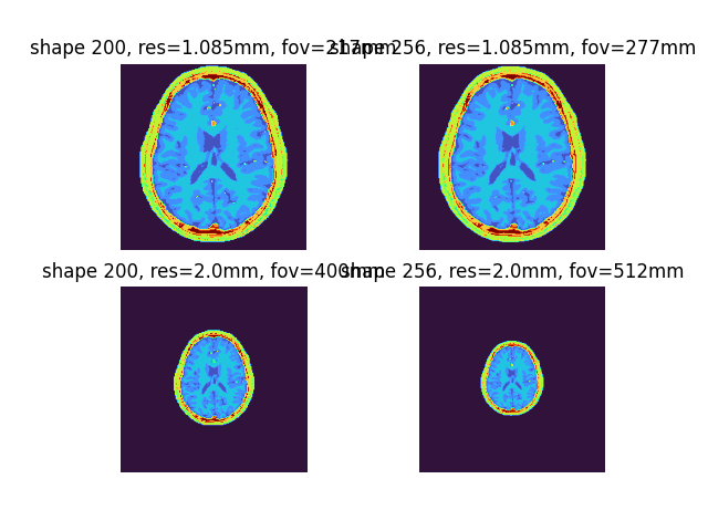
By default, Brainweb phantoms are interpolated to 1.085 mm isotropic resolution with a 200 isotropic matrix (217 mm iso FOV).

These can be adjusted using shape and output_res model:

1. shape will control the matrix size without affecting the resolution.

2. output_res will adjust the spatial resolution keeping the same (i.e., 200 iso) matrix

phantom2D = brainweb_phantom(ndim=2, subject=4)
phantom2D_mtx = brainweb_phantom(
    ndim=2, subject=4, shape=256
)  # can also be shape=(ny, nx)
phantom2D_res = brainweb_phantom(
    ndim=2, subject=4, output_res=2.0
)  # can also be output_res=(dy, dx)
phantom2D_mtx_res = brainweb_phantom(ndim=2, subject=4, shape=256, output_res=2.0)

print(phantom2D)
print(phantom2D_mtx)
print(phantom2D_res)
print(phantom2D_mtx_res)

fig4, ax4 = plt.subplots(2, 2)
ax4[0, 0].imshow(phantom2D, cmap="turbo"), ax4[0, 0].axis("off"), ax4[0, 0].set_title(
    "shape 200, res=1.085mm, fov=217mm"
)
ax4[0, 1].imshow(phantom2D_mtx, cmap="turbo"), ax4[0, 1].axis("off"), ax4[
    0, 1
].set_title("shape 256, res=1.085mm, fov=277mm")
ax4[1, 0].imshow(phantom2D_res, cmap="turbo"), ax4[1, 0].axis("off"), ax4[
    1, 0
].set_title("shape 200, res=2.0mm, fov=400mm")
ax4[1, 1].imshow(phantom2D_mtx_res, cmap="turbo"), ax4[1, 1].axis("off"), ax4[
    1, 1
].set_title("shape 256, res=2.0mm, fov=512mm")
plt.show()

Crisp Brainweb phantom with following properties:
Number of spatial dimensions: 2
Tissue properties: dict_keys(['M0', 'T1', 'T2', 'T2s', 'Chi'])
Matrix size: (200, 200)

Crisp Brainweb phantom with following properties:
Number of spatial dimensions: 2
Tissue properties: dict_keys(['M0', 'T1', 'T2', 'T2s', 'Chi'])
Matrix size: (256, 256)

Crisp Brainweb phantom with following properties:
Number of spatial dimensions: 2
Tissue properties: dict_keys(['M0', 'T1', 'T2', 'T2s', 'Chi'])
Matrix size: (200, 200)

Crisp Brainweb phantom with following properties:
Number of spatial dimensions: 2
Tissue properties: dict_keys(['M0', 'T1', 'T2', 'T2s', 'Chi'])
Matrix size: (256, 256)

The physical parameter of each tissue class are calculated by default for a field strength of 1.5 T.

This can be changed via the B0 argument:

# B0 strengths
B0 = [0.55, 1.5, 3.0, 7.0, 11.7, 13.3]  # field strengths in [T]

# Generate phantoms with different field strengths
phantomB0 = [
    brainweb_phantom(ndim=2, subject=4, B0=strength, segtype=False) for strength in B0
]

# Display
T1 = np.concatenate([phantom.T1 for phantom in phantomB0], axis=1)
T2 = np.concatenate([phantom.T2 for phantom in phantomB0], axis=1)
T2s = np.concatenate([phantom.T2s for phantom in phantomB0], axis=1)

fig5, ax5 = plt.subplots(3, 1)

im1 = ax5[0].imshow(T1, cmap="magma", vmax=5000)
ax5[0].axis("off"), ax5[0].set_title("T1 [ms]")
fig5.colorbar(im1, ax=ax5[0], fraction=0.046, pad=0.04)

im2 = ax5[1].imshow(T2, cmap="viridis", vmax=150)
ax5[1].axis("off"), ax5[1].set_title("T2 [ms]")
fig5.colorbar(im2, ax=ax5[1], fraction=0.046, pad=0.04)

im3 = ax5[2].imshow(T2s, cmap="viridis", vmax=100)
ax5[2].axis("off"), ax5[2].set_title("T2* [ms]")
fig5.colorbar(im3, ax=ax5[2], fraction=0.046, pad=0.04)

plt.tight_layout()
plt.show()

In addition to single pool model, we provide 3 multi-pool models:

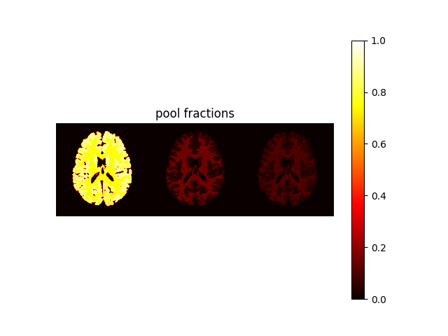
1. "mw-model": a two-pool model where free water is divided in two compartments, i.e., intra-/extra-cellular water (long T1 / T2) and myelin water (short T1 / T2). The model include chemical exchange between the two pools. Parameters are (MWF, T1, T2, k, chemshift).

2. "mt-model": a two-pool model consisting in free water and bound water. Free water includes both intra-/extra-cellular and myelin water (as in the single-pool model), while bound water corresponds to a macromolecular pool with the same T1 as the free water and no T2 (i.e., no transverse magnetiztion). The model include magnetization transfer between the two pools. Parameters are (MVF, T1, T2, k).

3. "mwmt-model": a three-pool model consisting in intra-/extra-cellular water, myelin water and bound water. The model include chemical exchange between the two free water pools and magnetizion transfer between myelin water and bound water. Parameters are (MWF, MVF, T1, T2, k).

Here we will display the latter, as it represents the most general case.

# model="single-pool" is the default, while "mw-model" and "mt-model" corresponds to cases 1. and 2.
phantom_multi = brainweb_phantom(ndim=2, subject=4, model="mwmt-model", segtype=False)

MWF corresponds to the myelin water fraction, while MVF to the bound water fraction. We assume that intra-extracellular water fraction = 1 - (MWF + MVF):

MWF = phantom_multi.MWF
MVF = phantom_multi.MVF
IEWF = (1 - (MWF + MVF)) * (MWF > 0)
weight = np.concatenate((IEWF, MWF, MVF), axis=1)

plt.figure()
plt.imshow(weight, vmin=0, vmax=1, cmap="hot"), plt.axis("off"), plt.title(
    "pool fractions"
), plt.colorbar()
plt.show()

T1 and T2 for the two free water pools are stacked along the first axis, with n=0 being the intra-/extra-cellular water (long T1 / T2) and n=1 being the myelin water (short T1 / T2):

T1 = np.concatenate((phantom_multi.T1[0], phantom_multi.T1[1]), axis=1)
T2 = np.concatenate((phantom_multi.T2[0], phantom_multi.T2[1]), axis=1)

fig6, ax6 = plt.subplots(2, 1)

im1 = ax6[0].imshow(T1, cmap="magma", vmax=1500)
ax6[0].axis("off"), ax6[0].set_title("T1 [ms]")
fig6.colorbar(im1, ax=ax6[0], fraction=0.046, pad=0.04)

im2 = ax6[1].imshow(T2, cmap="viridis", vmax=150)
ax6[1].axis("off"), ax6[1].set_title("T2 [ms]")
fig6.colorbar(im2, ax=ax6[1], fraction=0.046, pad=0.04)

<matplotlib.colorbar.Colorbar object at 0x7f3dc0ad2dd0>

k represent the non-directional exchange rates in [Hz], with n=0 being the chemical exchange rate between the two free water pools and n=1 being magnetization transfer rate between the myelin and bound water:

k = np.concatenate((phantom_multi.k[0], phantom_multi.k[1]), axis=1)

plt.figure()
plt.imshow(k, cmap="hot"), plt.axis("off"), plt.title(
    "exchange rate [Hz]"
), plt.colorbar()
plt.show()

Similarly to the single pool model, mrtwin supports "fuzzy" and "crisp" segmentations.

Caching mechanism

To reduce loading times, mrtwin implements a caching mechanism.

If cache argument is set to True (default behaviour), each phantom segmentation (identified by the number of spatial dimensions, tissue model, segmentation type, matrix shape and resolution) is saved on the disk in npy format.

The path is selected according to the following hierachy (inspired by brainweb-dl):

1. User-specific argument (cache_dir)

2. MRTWIN_DIR environment variable

3. ~/.cache/mrtwin folder

On top of that, the underlying Brainweb fuzzy segmentations at the original resolution are stored (via brainweb-dl) with the following hierachy:

1. User-specific argument (brainweb_dir)

2. BRAINWEB_DIR environment variable

3. ~/.cache/brainweb folder

The cached files can be forcibly overwritten by setting the force argument to True (default: False).

N.B.: currently, force=True will both force re-downloading brainweb segmentation and the subsequent interpolations and resizing required to obtain the desired shape and resolution.

Disabling SSL verification (not recommended)

If you encounter some issue in downloading, SSL verification can be disabled by setting verify to False (default: True). It is advised however to solve the problem on your machine side (updating the certificate).