Open Science CBS Neuroimaging Repository Phantom

Example of Open Science CBS Neuroimaging Repository phantom creation.

This dataset consists of an additional processing of the dataset created by Tardif et al. [1], and stored in a Open Science Framework (OSF) repository.

This examples show how to generate numerical phantoms based on the Brainweb dataset.

References

[1] Tardif CL, Schäfer A, Trampel R, Villringer A, Turner R, Bazin PL. Open Science CBS Neuroimaging Repository: Sharing ultra-high-field MR images of the brain. Neuroimage. 2016 Jan 1;124(Pt B):1143-1148. doi: 10.1016/j.neuroimage.2015.08.042. Epub 2015 Aug 25. PMID: 26318051.

import matplotlib.pyplot as plt
import numpy as np

from mrtwin import osf_phantom

Basic Usage

The Open Science CBS Neuroimaging database (hereafter referred to as OSF) consists of a set of 20 normal brains (ids equal to [1-4, 6, 8-15, 17, 19, 22-23, 25, 27-28]) at a nominal 0.5 mm isotropic and a shape of (nz, ny, nx) = (454, 544, 454).

A digital OSF phantom can be created as:

phantom = osf_phantom(ndim=2, subject=1)  # 2D phantom

Here, without loss of generality, we use a single-slice 2D phantom. A 3D phantom can be generated by setting ndim=3.

The (M0, T1, T2, T2*, Chi) properties of the phantom can be direcly accessed as:

fig1, ax1 = plt.subplots(1, 5)

im0 = ax1[0].imshow(phantom.M0, cmap="gray", vmin=0)
ax1[0].axis("off"), ax1[0].set_title("M0 [a.u.]")
fig1.colorbar(im0, ax=ax1[0], fraction=0.046, pad=0.04)

im1 = ax1[1].imshow(phantom.T1, cmap="magma", vmin=0)
ax1[1].axis("off"), ax1[1].set_title("T1 [ms]")
fig1.colorbar(im1, ax=ax1[1], fraction=0.046, pad=0.04)

im2 = ax1[2].imshow(phantom.T2, cmap="viridis", vmin=0, vmax=250)
ax1[2].axis("off"), ax1[2].set_title("T2 [ms]")
fig1.colorbar(im2, ax=ax1[2], fraction=0.046, pad=0.04)

im3 = ax1[3].imshow(phantom.T2s, cmap="viridis", vmin=0, vmax=250)
ax1[3].axis("off"), ax1[3].set_title("T2* [ms]")
fig1.colorbar(im3, ax=ax1[3], fraction=0.046, pad=0.04)

im4 = ax1[4].imshow(phantom.Chi, cmap="gray")
ax1[4].axis("off"), ax1[4].set_title("Chi")
fig1.colorbar(im4, ax=ax1[4], fraction=0.046, pad=0.04)

plt.tight_layout()
plt.show()

If required, the properties dictionary can be directly accessed as phantom.properties, e.g., to be passed as **kwargs to a simulator routine.

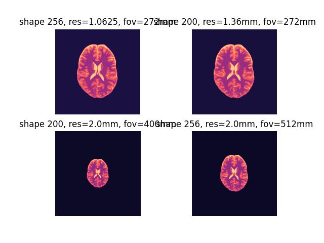
By default, OSF phantoms are interpolated to 1.0625 mm isotropic resolution with a 256 isotropic matrix (272 mm iso FOV).

These can be adjusted using shape and output_res model:

1. shape will control the matrix size without affecting the resolution.

2. output_res will adjust the spatial resolution keeping the same (i.e., 200 iso) matrix

phantom = osf_phantom(ndim=2, subject=1)
phantom_mtx = osf_phantom(ndim=2, subject=1, shape=200)  # can also be shape=(ny, nx)
phantom_res = osf_phantom(
    ndim=2, subject=1, output_res=2.0
)  # can also be output_res=(dy, dx)
phantom_mtx_res = osf_phantom(ndim=2, subject=1, shape=200, output_res=2.0)

print(phantom)
print(phantom_mtx)
print(phantom_res)
print(phantom_mtx_res)

fig2, ax2 = plt.subplots(2, 2)
ax2[0, 0].imshow(phantom.T1, cmap="magma"), ax2[0, 0].axis("off"), ax2[0, 0].set_title(
    "shape 256, res=1.0625, fov=272mm"
)
ax2[0, 1].imshow(phantom_mtx.T1, cmap="magma"), ax2[0, 1].axis("off"), ax2[
    0, 1
].set_title("shape 200, res=1.36mm, fov=272mm")
ax2[1, 0].imshow(phantom_res.T1, cmap="magma"), ax2[1, 0].axis("off"), ax2[
    1, 0
].set_title("shape 200, res=2.0mm, fov=400mm")
ax2[1, 1].imshow(phantom_mtx_res.T1, cmap="magma"), ax2[1, 1].axis("off"), ax2[
    1, 1
].set_title("shape 256, res=2.0mm, fov=512mm")
plt.show()

Dense OSF phantom with following properties:
Number of spatial dimensions: 2
Tissue properties: dict_keys(['M0', 'T1', 'T2', 'T2s', 'Chi'])
Matrix size: (256, 256)

Dense OSF phantom with following properties:
Number of spatial dimensions: 2
Tissue properties: dict_keys(['M0', 'T1', 'T2', 'T2s', 'Chi'])
Matrix size: (200, 200)

Dense OSF phantom with following properties:
Number of spatial dimensions: 2
Tissue properties: dict_keys(['M0', 'T1', 'T2', 'T2s', 'Chi'])
Matrix size: (256, 256)

Dense OSF phantom with following properties:
Number of spatial dimensions: 2
Tissue properties: dict_keys(['M0', 'T1', 'T2', 'T2s', 'Chi'])
Matrix size: (200, 200)

The physical parameter of each tissue class are reported by default for a field strength of 3.0 T.

This can be changed via the B0 argument:

# B0 strengths
B0 = [0.55, 1.5, 3.0, 7.0, 11.7, 13.3]  # field strengths in [T]

# Generate phantoms with different field strengths
phantomB0 = [osf_phantom(ndim=2, subject=1, B0=strength) for strength in B0]

# Display
T1 = np.concatenate([phantom.T1 for phantom in phantomB0], axis=1)
T2 = np.concatenate([phantom.T2 for phantom in phantomB0], axis=1)
T2s = np.concatenate([phantom.T2s for phantom in phantomB0], axis=1)

fig5, ax5 = plt.subplots(3, 1)

im1 = ax5[0].imshow(T1, cmap="magma", vmin=0, vmax=5000)
ax5[0].axis("off"), ax5[0].set_title("T1 [ms]")
fig5.colorbar(im1, ax=ax5[0], fraction=0.046, pad=0.04)

im2 = ax5[1].imshow(T2, cmap="viridis", vmin=0, vmax=250)
ax5[1].axis("off"), ax5[1].set_title("T2 [ms]")
fig5.colorbar(im2, ax=ax5[1], fraction=0.046, pad=0.04)

im3 = ax5[2].imshow(T2s, cmap="viridis", vmin=0, vmax=250)
ax5[2].axis("off"), ax5[2].set_title("T2* [ms]")
fig5.colorbar(im3, ax=ax5[2], fraction=0.046, pad=0.04)

plt.tight_layout()
plt.show()

In this case, T1 and T2* are extrapolated from their 3.0 T values.

Caching mechanism

To reduce loading times, mrtwin implements a caching mechanism.

If cache argument is set to True (default behaviour), each phantom segmentation (identified by the number of spatial dimensions, matrix shape and resolution) is saved on the disk in npy format.

The path is selected according to the following hierachy (inspired by brainweb-dl):

1. User-specific argument (cache_dir)

2. MRTWIN_DIR environment variable

3. ~/.cache/mrtwin folder

Disabling SSL verification (not recommended)

If you encounter some issue in downloading, SSL verification can be disabled by setting verify to False (default: True). It is advised however to solve the problem on your machine side (updating the certificate).