Gradien System Response Function Generation

Example of Gradien System Response Function (GIRF) generation.

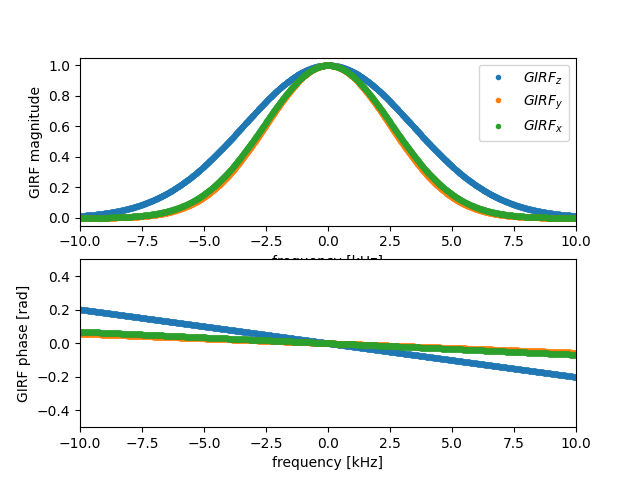
The GIRF is approximated as a complex-valued array, whose magnitude (modeled) as a Gaussian of the specified Full Width Half Maximum, which dampens high-frequency components of the k-space trajectory, and whose phase is a linear ramp representing a non-integer shift of the waveform.

The response is modeled independently for the three physical axes z, y, x.

import matplotlib.pyplot as plt
import numpy as np

from mrtwin import generate_girf

Typical values for gradient raster times dt are around 5-10 us (GE: 4us; Siemens: 10us; Philips: 6.4us)

GIRF magnitudes Full Width Half Maximum are on the order of 5 kHz, while gradient delays are on the order of 1us.

GIRF for the x and y axes are more similar to each other when compared to z axes.

Given a GIRF measurement time window of 100ms, function parameters are as follows:

dt = 4e-6  # assume GE raster time
N = int(100e-3 // dt)  # approximate number of points
fwhm = (8.0e3, 5.9e3, 6.1e3)
delay = (3.2e-6, 0.9e-6, 1.1e-6)

Given these parameters, GIRF can be computed as

freqs, girf = generate_girf(dt, N, fwhm, delay)

fig, ax = plt.subplots(2, 1)
ax[0].plot(freqs * 1e-3, np.abs(girf).T, "."), ax[0].set_xlim([-10, 10]), ax[0].legend(
    ["$GIRF_z$", "$GIRF_y$", "$GIRF_x$"]
), ax[0].set(xlabel="frequency [kHz]", ylabel="GIRF magnitude")
ax[1].plot(freqs * 1e-3, np.angle(girf).T, "."), ax[1].set_xlim([-10, 10]), ax[
    1
].set_ylim([-0.5, 0.5]), ax[1].set(xlabel="frequency [kHz]", ylabel="GIRF phase [rad]")

([<matplotlib.lines.Line2D object at 0x7f3dc0bf8fa0>, <matplotlib.lines.Line2D object at 0x7f3dc0bf9f30>, <matplotlib.lines.Line2D object at 0x7f3dc0bfb970>], (-10.0, 10.0), (-0.5, 0.5), [Text(0.5, 23.52222222222222, 'frequency [kHz]'), Text(31.222222222222214, 0.5, 'GIRF phase [rad]')])