Static Field Simulation

Example of static field generation.

This examples show how to generate a static field (i.e., B0) map starting from the object susceptibility distribution.

The static field is written as the following convolution (performed as a pointwise multiplication in the Fourier space):

\[\mathbf{B}(\mathbf{r}) = \mathbf{B_0} \cdot \mathcal{F}^{-1} \left[ \chi(\mathbf{k}) \cdot D(\mathbf{k}) \right]\]

where \(\chi(\mathbf{k})\) is the Fourier transform of susceptibility spatial distribution and \(D(\mathbf{k})\) is the dipole kernel defined by:

\[D(\mathbf{r}) = \left(\frac{1}{3} - \frac{k^2_z}{\lvert \textbf{k} \rvert}\right)\]

import matplotlib.pyplot as plt
import numpy as np

from mrtwin import shepplogan_phantom, b0field

Generate susceptibility distribution

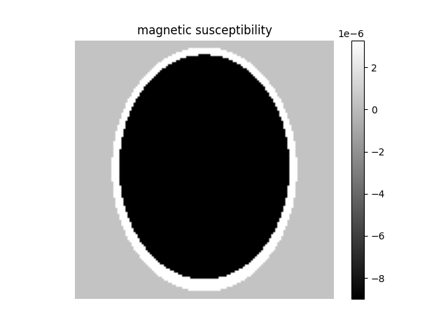
First, we generate a 3D Shepp-Logan phantom:

phantom = shepplogan_phantom(ndim=3, shape=128, segtype=False)

# Get susceptibility
chi = phantom.Chi

plt.figure()
plt.imshow(chi[64], cmap="gray"), plt.axis("off"), plt.colorbar(), plt.title(
    "magnetic susceptibility"
)
plt.show()

Basic Usage

Starting from the susceptibility distribution, we can generate the corresponding static field perturbation as:

b0map = b0field(chi)

plt.figure()
plt.imshow(b0map[64], cmap="turbo", vmin=-300, vmax=300), plt.axis(
    "off"
), plt.colorbar(), plt.title("B0 map [Hz]")
plt.show()

Optionally, we can provide a mask of the object to exclude the background:

mask = phantom.M0 != 0.0
b0map = b0field(chi, mask=mask)

plt.figure()
plt.imshow(b0map[64], cmap="turbo", vmin=-300, vmax=300), plt.axis(
    "off"
), plt.colorbar(), plt.title("masked B0 map [Hz]")
plt.show()

The static field map calculated by default for a field strength of 1.5 T.

This can be changed via the B0 argument:

# B0 strengths
B0 = [0.55, 1.5, 3.0, 7.0, 11.7, 13.3]  # field strengths in [T]

# Generate phantoms with different field strengths
b0maps = [b0field(chi, B0=strength) for strength in B0]

# Display
b0map = np.concatenate([b0map[64] for b0map in b0maps], axis=1)

plt.figure()
plt.imshow(b0map, cmap="turbo", vmin=-300, vmax=300), plt.axis(
    "off"
), plt.colorbar(), plt.title("B0 map [Hz]")
plt.show()

As an alternative, we can force a specific B0 offset range using the b0range argument as:

b0map = b0field(chi, b0range=(-500, 500))

plt.figure()
plt.imshow(b0map[64], cmap="turbo", vmin=-300, vmax=300), plt.axis(
    "off"
), plt.colorbar(), plt.title("B0 map [Hz]")
plt.show()