Coil Sensitivity Simulation

Example of coil sensitivity map generation.

This examples show how to generate coil sensitivity maps for a multi-channel receiver array.

import matplotlib.pyplot as plt
import numpy as np

from mrtwin import sensmap

plt.rcParams["image.cmap"] = "gray"

Basic Usage

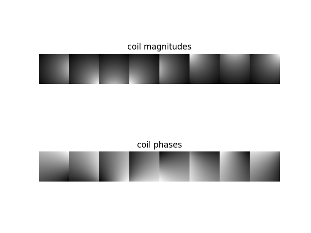
Two- and three-dimensional coil sensitivity maps can be generated providing (nc, ny, nx) and (nc, nz, ny, nx) shaped tuple as a shape argument to sensmap routine, respectively:

smap2D = sensmap(shape=(8, 200, 200))  # 8 channels; (200, 200) matrix
print(smap2D.shape)

smap3D = sensmap(shape=(8, 128, 128, 128))  # 8 channels; (128, 128, 128) matrix
print(smap3D.shape)

display_magn = np.concatenate([np.abs(smap) for smap in smap2D], axis=1)
display_phase = np.concatenate([np.angle(smap) for smap in smap2D], axis=1)

fig1, ax1 = plt.subplots(2, 1)
ax1[0].imshow(display_magn), ax1[0].axis("off"), ax1[0].set_title("coil magnitudes")
ax1[1].imshow(display_phase), ax1[1].axis("off"), ax1[1].set_title("coil phases")
plt.show()

(8, 200, 200)
(8, 128, 128, 128)

Advanced Options

The sensitivity maps can be altered by modifying several parameters:

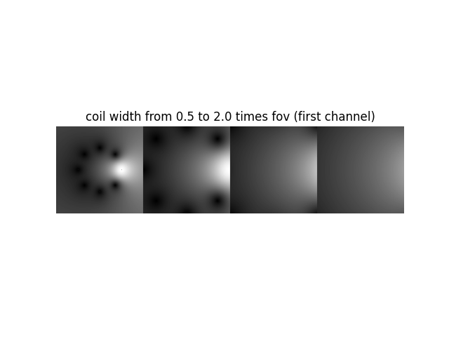
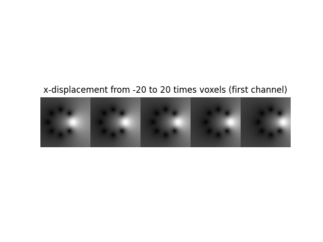
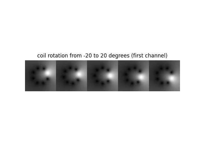
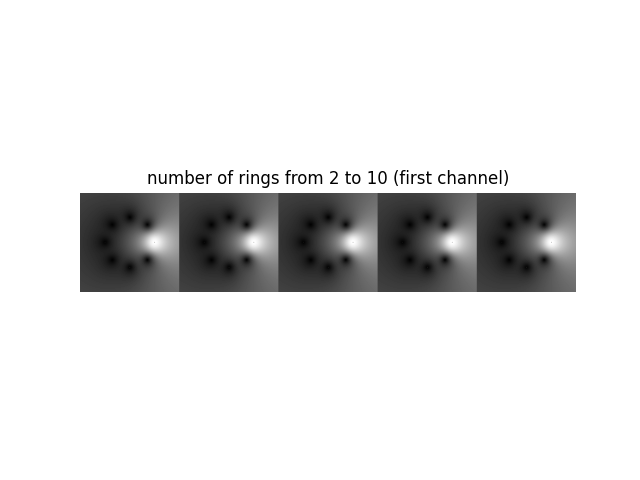
1. coil_width: width of the coil (with respect to FOV).

2. shift: displacement of the center (in units of voxels).

3. dphi: bulk rotation of the coil (in [deg]).

4. nrings: number of rings for a cylindrical hardware setup.

Without loss of generality, we show examples for 2D sensitivities:

Coil width

widths = [0.5, 1.0, 1.5, 2.0]
smap2D = [
    sensmap(shape=(8, 200, 200), coil_width=w)[0] for w in widths
]  # only show first channel

display = np.concatenate(smap2D, axis=1)

plt.figure()
plt.imshow(abs(display)), plt.axis("off"), plt.title(
    "coil width from 0.5 to 2.0 times fov (first channel)"
)
plt.show()

Center shift

dx = [-20, -10, 0, 10, 20]
smap2D = [
    sensmap(shape=(8, 200, 200), shift=(0, x), coil_width=0.5)[0] for x in dx
]  # for 3D, it would be shift=(dz, dy, dx)

display = np.concatenate(smap2D, axis=1)

plt.figure()
plt.imshow(abs(display)), plt.axis("off"), plt.title(
    "x-displacement from -20 to 20 times voxels (first channel)"
)
plt.show()

Rotation

phi = [-20, -10, 0, 10, 20]
smap2D = [sensmap(shape=(8, 200, 200), dphi=angle, coil_width=0.5)[0] for angle in phi]

display = np.concatenate(smap2D, axis=1)

plt.figure()
plt.imshow(abs(display)), plt.axis("off"), plt.title(
    "coil rotation from -20 to 20 degrees (first channel)"
)
plt.show()

Number of rings

nrings = [2, 4, 6, 8, 10]
smap2D = [sensmap(shape=(8, 200, 200), nrings=n, coil_width=0.5)[0] for n in nrings]

display = np.concatenate(smap2D, axis=1)

plt.figure()
plt.imshow(abs(display)), plt.axis("off"), plt.title(
    "number of rings from 2 to 10 (first channel)"
)
plt.show()

Caching mechanism

To reduce loading times, mrtwin implements a caching mechanism.

If cache argument is set to True (default behaviour for ndim=3), each sensitivity map segmentation (identified by the number of channels, matrix size, shift, rotation angle and number of rings) is saved on the disk in npy format.

The path is selected according to the following hierachy (inspired by brainweb-dl):

1. User-specific argument (cache_dir)

2. MRTWIN_DIR environment variable

3. ~/.cache/mrtwin folder