Transmit Field Simulation

Example of transmit field (i.e., B1+) map generation.

This examples show how to generate coil sensitivity maps for a single or multi-channel transmit array.

import matplotlib.pyplot as plt
import numpy as np

from mrtwin import b1field

plt.rcParams["image.cmap"] = "hot"

Basic Usage

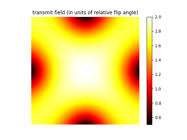
Two- and three-dimensional transmit field maps can be generated providing (ny, nx) and (nz, ny, nx) shaped tuple as a shape argument to b1field routine, respectively:

b1map2D = b1field(shape=(200, 200))  # (200, 200) matrix
print(b1map2D.shape)

b1map3D = b1field(shape=(128, 128, 128))  # (128, 128, 128) matrix
print(b1map3D.shape)

plt.figure()
plt.imshow(b1map2D), plt.axis("off"), plt.colorbar(), plt.title(
    "transmit field (in units of relative flip angle)"
)
plt.show()

(200, 200)
(128, 128, 128)

The transmit field maps are generated with a relative flip angle variation between 0.8 and 1.2 (e.g., 3T systems).

This can be changed via the b1range argument:

b1map2D = b1field(shape=(200, 200), b1range=(0.5, 2.0))

plt.figure()
plt.imshow(b1map2D), plt.axis("off"), plt.colorbar(), plt.title(
    "transmit field with b1range between 0.5 and 2.0"
)
plt.show()

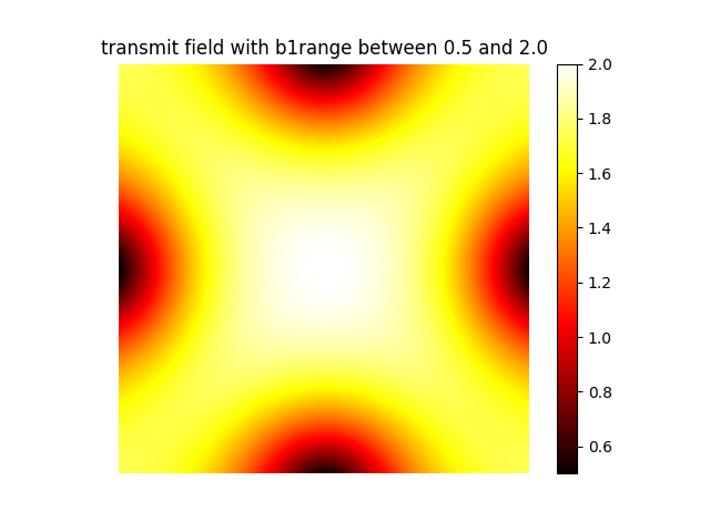
This can be used e.g., to simulate field maps for higher fields (e.g., 7T systems).

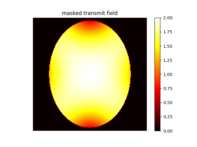
Optionally, we can provide a mask of the object to exclude the background when calculating the field rescaling:

from mrtwin import shepplogan_phantom

mask = shepplogan_phantom(ndim=2, shape=(200, 200), segtype=False).M0 != 0.0
b1map2D = b1field(shape=(200, 200), mask=mask)

plt.figure()
plt.imshow(b1map2D), plt.axis("off"), plt.colorbar(), plt.title("masked transmit field")
plt.show()

Advanced Options

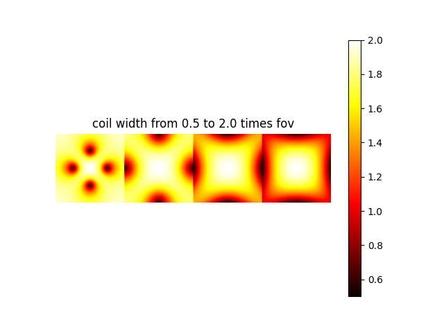
The sensitivity maps can be altered by modifying several parameters:

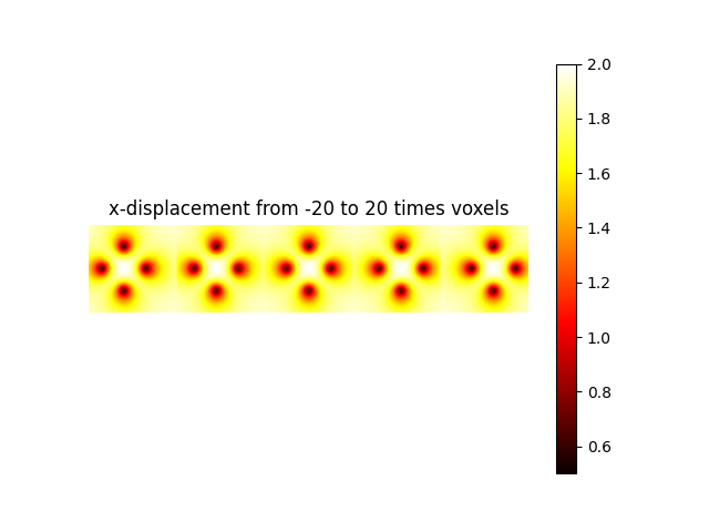
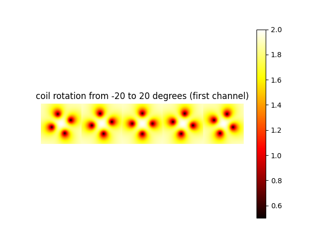
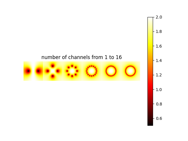
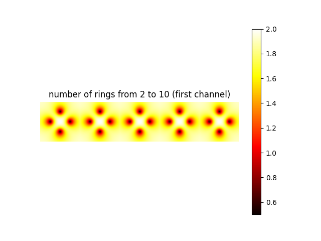
1. coil_width: width of the coil (with respect to FOV).

2. shift: displacement of the center (in units of voxels).

3. dphi: bulk rotation of the coil (in [deg]).

4. ncoils: number of transmit channels in the transmit array.

5. nrings: number of rings for a cylindrical hardware setup.

Without loss of generality, we show examples for 2D sensitivities:

Coil width

widths = [0.5, 1.0, 1.5, 2.0]
b1map2D = [
    b1field(shape=(200, 200), coil_width=w) for w in widths
]  # only show first channel

display = np.concatenate(b1map2D, axis=1)

plt.figure()
plt.imshow(abs(display)), plt.axis("off"), plt.colorbar(), plt.title(
    "coil width from 0.5 to 2.0 times fov"
)
plt.show()

Center shift

dx = [-20, -10, 0, 10, 20]
b1map2D = [
    b1field(shape=(200, 200), shift=(0, x), coil_width=0.5) for x in dx
]  # for 3D, it would be shift=(dz, dy, dx)

display = np.concatenate(b1map2D, axis=1)

plt.figure()
plt.imshow(abs(display)), plt.axis("off"), plt.colorbar(), plt.title(
    "x-displacement from -20 to 20 times voxels"
)
plt.show()

Rotation

phi = [-20, -10, 0, 10, 20]
b1map2D = [b1field(shape=(200, 200), dphi=angle, coil_width=0.5) for angle in phi]

display = np.concatenate(b1map2D, axis=1)

plt.figure()
plt.imshow(abs(display)), plt.axis("off"), plt.colorbar(), plt.title(
    "coil rotation from -20 to 20 degrees (first channel)"
)
plt.show()

Number of rings

ncoils = [1, 2, 4, 8, 16, 32]
b1map2D = [b1field(shape=(200, 200), ncoils=n, coil_width=0.5) for n in ncoils]

display = np.concatenate(b1map2D, axis=1)

plt.figure()
plt.imshow(abs(display)), plt.axis("off"), plt.colorbar(), plt.title(
    "number of channels from 1 to 16"
)
plt.show()

Number of rings

nrings = [2, 4, 6, 8, 10]
b1map2D = [b1field(shape=(200, 200), nrings=n, coil_width=0.5) for n in nrings]

display = np.concatenate(b1map2D, axis=1)

plt.figure()
plt.imshow(abs(display)), plt.axis("off"), plt.colorbar(), plt.title(
    "number of rings from 2 to 10 (first channel)"
)
plt.show()

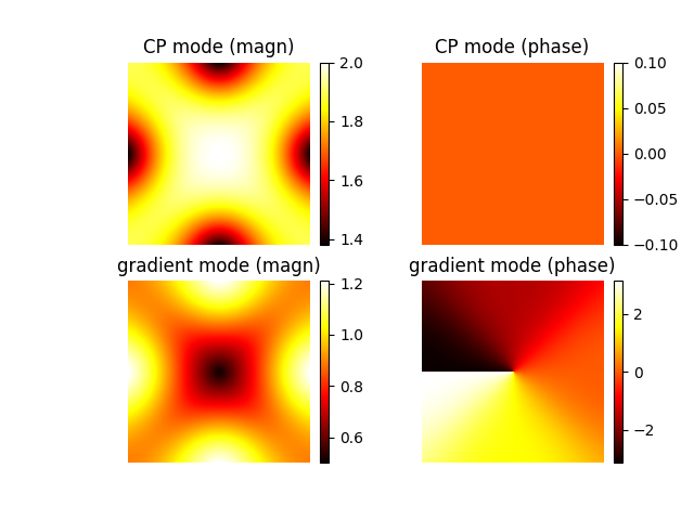
Multiple Transmit Modes

By default, the sensitivities from each transmit channel are combined in quadrature mode.

With mrtwin, multiple orthogonal modes can be simulated by nmodes argument. For example, CP mode and gradient modes (e.g., for static pTx) can be obtained as:

b1map = b1field((200, 200), nmodes=2)  # b1map[0] is CP, b1map[1] is gradient mode.

In this case, b1map will be a (nmodes, *shape) np.ndarray, the different modes being stacked along the first axis:

fig, ax = plt.subplots(2, 2)
im0 = ax[0, 0].imshow(np.abs(b1map[0]))
ax[0, 0].axis("off"), ax[0, 0].set_title("CP mode (magn)")
fig.colorbar(im0, ax=ax[0, 0], fraction=0.046, pad=0.04)

im1 = ax[0, 1].imshow(np.angle(b1map[0]))
ax[0, 1].axis("off"), ax[0, 1].set_title("CP mode (phase)")
fig.colorbar(im1, ax=ax[0, 1], fraction=0.046, pad=0.04)

im2 = ax[1, 0].imshow(np.abs(b1map[1]))
ax[1, 0].axis("off"), ax[1, 0].set_title("gradient mode (magn)")
fig.colorbar(im2, ax=ax[1, 0], fraction=0.046, pad=0.04)

im3 = ax[1, 1].imshow(np.angle(b1map[1]))
ax[1, 1].axis("off"), ax[1, 1].set_title("gradient mode (phase)")
fig.colorbar(im3, ax=ax[1, 1], fraction=0.046, pad=0.04)
plt.show()

Caching mechanism

To reduce loading times, mrtwin implements a caching mechanism.

If cache argument is set to True (default behaviour for ndim=3), each transmit field map segmentation (identified by the number of channels, number of modes, matrix size, shift, rotation angle, number of rings, b1 range and masking flag) is saved on the disk in npy format.

The path is selected according to the following hierachy (inspired by brainweb-dl):

1. User-specific argument (cache_dir)

2. MRTWIN_DIR environment variable

3. ~/.cache/mrtwin folder