b0field#

mrtwin.b0field(chi, b0range=None, mask=None, B0=1.5)[source]#

Simulate inhomogeneous B0 fields.

Output field units is [Hz]. The field is created by convolving the dipole kernel with an input magnetic susceptibility map.

Parameters:

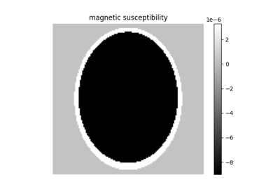
chi (np.ndarray) – Object magnetic susceptibility map in [ppb] of shape (ny, nx) (2D) or (nz, ny, nx) (3D).
b0range (Sequence[float] | None, optional) – Range of B0 field in [Hz]. The default is None (do not force a range).
mask (np.ndarray, optional) – Region of support of the object of shape (ny, nx) (2D) or (nz, ny, nx) (3D). The default is None.
B0 (float, optional) – Static field strength in [T]. Used to compute B0 scaling (assuming 1H imaging) if b0range is not provided. The default is 1.5.

Returns:

B0map – Spatially varying B0 maps of shape (ny, nx) (2D) or (nz, ny, nx) (3D) in [Hz], arising from the object susceptibility.

Return type:

np.ndarray

Example

>>> from mrtwin import shepplogan_phantom, b0field

We can generate a 2D B0 field map of shape (ny=128, nx=128) starting from a magnetic susceptibility distribution:

>>> chi = shepplogan_phantom(2, 128, segtype=False).Chi
>>> b0map = b0field(chi)

B0 values range can be specified using b0range argument:

>>> b0map = b0field(chi, b0range=(-500, 500))

Examples using `mrtwin.b0field`#