Automatic differentiation

This example showcase the automatic differentiation capabilities of the framework.

First, we will import the required packages:

import warnings

warnings.filterwarnings("ignore")

from functools import partial

import numpy as np
import torch

from torch.func import jacrev

import matplotlib.pyplot as plt
import time

We will show how to use automatic differentiation to automatically compute Cramer Rao Lower Bound.

This can be used as a cost function to optimize acquisition schedules, for example for quantitative MRI

We’ll focuse on a simple Fast Spin Echo acquisition:

import torchsim

Cramer Rao Lower Bound is defined as the diagonal of the inverse of Fisher information matrix. This can be computed as

def calculate_crlb(grad, W=None, weight=1.0):
    if len(grad.shape) == 1:
        grad = grad[None, :]

    if W is None:
        W = torch.eye(grad.shape[0], dtype=grad.dtype, device=grad.device)

    J = torch.stack((grad.real, grad.imag), axis=0)  # (nparams, nechoes)
    J = J.permute(2, 1, 0)

    # calculate Fischer information matrix
    In = torch.einsum("bij,bjk->bik", J, J.permute(0, 2, 1))
    I = In.sum(axis=0)  # (nparams, nparams)

    # Invert
    return torch.trace(torch.linalg.inv(I) * W).real * weight

notice that we used the trace as a cost function. For optimization, we need the gradient of this cost wrt sequence parameters.

This can be obtained as:

def _crlb_cost(ESP, T1, T2, flip):

    # calculate signal and derivative
    _, grad = torchsim.fse_sim(flip=flip, ESP=ESP, T1=T1, T2=T2, diff="T2")

    # calculate cost
    return calculate_crlb(grad)


def crlb_cost(flip, ESP, T1, T2):
    flip = torch.as_tensor(flip, dtype=torch.float32)
    flip.requires_grad = True

    # get partial function
    _cost = partial(_crlb_cost, ESP, T1, T2)
    _dcost = jacrev(_cost)

    return _cost(flip).detach().cpu().numpy(), _dcost(flip).detach().cpu().numpy()

As reference, we compute derivatives via finite differences approximation. This is inaccurate, but as easy to implement as automatic differentiation:

def fse_finitediff_grad(flip, ESP, T1, T2):
    sig = torchsim.fse_sim(flip=flip, ESP=ESP, T1=T1, T2=T2)

    # numerical derivative
    dt = 1.0
    dsig = torchsim.fse_sim(flip=flip, ESP=ESP, T1=T1, T2=T2 + dt)

    return sig, (dsig - sig) / dt


def _crlb_finitediff_cost(ESP, T1, T2, flip):

    # calculate signal and derivative
    _, grad = fse_finitediff_grad(flip, ESP, T1, T2)

    # calculate cost
    return calculate_crlb(grad).cpu().detach().numpy()


def crlb_finitediff_cost(flip, ESP, T1, T2):

    # initial cost
    cost0 = _crlb_finitediff_cost(ESP, T1, T2, flip)
    dcost = []

    for n in range(len(flip)):
        # get angles
        angles = flip.copy()
        angles[n] += 1.0
        dcost.append(_crlb_finitediff_cost(ESP, T1, T2, angles))

    return cost0, (np.asarray(dcost) - cost0)

Now, we can compute optimization for a specific tissue.

We assume T1 = 1000.0 ms and T2 = 100.0 ms:

t1 = 1000.0
t2 = 100.0

Let’s compute CRLB for a constant 180.0 refocusing schedule, preceded by a ramp:

angles = np.ones(96) * 60.0
esp = 5.0  # ms

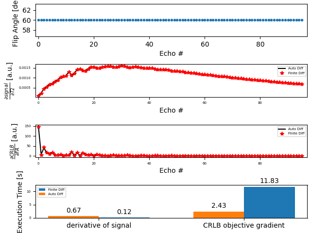
Run and plot timings:

tstart = time.time()
sig0, grad0 = fse_finitediff_grad(angles, esp, t1, t2)
tstop = time.time()
tgrad0 = tstop - tstart

tstart = time.time()
sig, grad = torchsim.fse_sim(flip=angles, ESP=esp, T1=t1, T2=t2, diff="T2")
tstop = time.time()
tgrad = tstop - tstart

# cost and derivative
tstart = time.time()
cost0, dcost0 = crlb_finitediff_cost(angles, esp, t1, t2)
tstop = time.time()
tcost0 = tstop - tstart

tstart = time.time()
cost, dcost = crlb_cost(angles, esp, t1, t2)
tstop = time.time()
tcost = tstop - tstart

fsz = 10
plt.figure()
plt.subplot(4, 1, 1)
plt.rcParams.update({"font.size": 0.5 * fsz})
plt.plot(angles, ".")
plt.xlabel("Echo #", fontsize=fsz)
plt.xlim([-1, 97])
plt.ylabel("Flip Angle [deg]", fontsize=fsz)

plt.subplot(4, 1, 2)
plt.rcParams.update({"font.size": 0.5 * fsz})
plt.plot(abs(grad), "-k"), plt.plot(abs(grad0), "*r")
plt.xlabel("Echo #", fontsize=fsz)
plt.xlim([-1, 97])
plt.ylabel(r"$\frac{\partial signal}{\partial T2}$ [a.u.]", fontsize=fsz)
plt.legend(
    [
        "Auto Diff",
        "Finite Diff",
    ]
)

plt.subplot(4, 1, 3)
plt.rcParams.update({"font.size": 0.5 * fsz})
plt.plot(abs(dcost), "-k"), plt.plot(abs(dcost0), "*r")
plt.xlabel("Echo #", fontsize=fsz)
plt.xlim([-1, 97])
plt.ylabel(r"$\frac{\partial CRLB}{\partial FA}$ [a.u.]", fontsize=fsz)
plt.legend(["Auto Diff", "Finite Diff"])

plt.subplot(4, 1, 4)
labels = ["derivative of signal", "CRLB objective gradient"]
time_finite = [round(tgrad0, 2), round(tcost0, 2)]
time_auto = [round(tgrad, 2), round(tcost, 2)]

x = np.arange(len(labels))  # the label locations
width = 0.35  # the width of the bars
rects1 = plt.bar(x + width / 2, time_finite, width, label="Finite Diff")
rects2 = plt.bar(x - width / 2, time_auto, width, label="Auto Diff")

# Add some text for labels, title and custom x-axis tick labels, etc.
plt.ylabel("Execution Time [s]", fontsize=fsz)
plt.xticks(x, labels, fontsize=fsz)
plt.legend()

plt.bar_label(rects1, padding=3, fontsize=fsz)
plt.bar_label(rects2, padding=3, fontsize=fsz)
plt.tight_layout()