Custom Simulator

This example shows how to use TorchSim to implement a simulator.

First, we want to implement the simulation engine. Parallelization and automatic differentiation are abstracted away from the user, which can focus on implementing single-voxel simulation.

We begin with the necessary imports:

import warnings

warnings.filterwarnings("ignore")

import numpy as np
import torch

from torchsim import base
from torchsim import epg

Defining the model

The model can be derived by base.AbstractModel as:

class SSFPMRFModel(base.AbstractModel):
    """Class to simulate inversion-prepared (variable flip angle) SSFP."""

    @base.autocast
    def set_properties(self, T1, T2):
        self.properties.T1 = T1
        self.properties.T2 = T2

    @base.autocast
    def set_sequence(self, flip, TR):
        self.sequence.flip = torch.pi * flip / 180.0
        self.sequence.TR = TR * 1e-3  # ms -> s

    @staticmethod
    def _engine(T1, T2, flip, TR):
        # Prepare relaxation parameters
        R1, R2 = 1e3 / T1, 1e3 / T2

        # Prepare EPG states matrix
        states = epg.states_matrix(
            device=R1.device,
            nstates=10,
        )

        # Prepare relaxation operator for sequence loop
        E1, rE1 = epg.longitudinal_relaxation_op(R1, TR)
        E2 = epg.transverse_relaxation_op(R2, TR)

        # Get number of shots
        nshots = len(flip)

        # Initialize signal
        signal = []

        # Apply inversion
        states = epg.adiabatic_inversion(states)

        # Scan loop
        for p in range(nshots):
            RF = epg.rf_pulse_op(flip[p])

            # Apply RF pulse
            states = epg.rf_pulse(states, RF)

            # Record signal
            signal.append(epg.get_signal(states))

            # Evolve
            states = epg.longitudinal_relaxation(states, E1, rE1)
            states = epg.transverse_relaxation(states, E2)
            states = epg.shift(states)

        return torch.stack(signal)

With this definition, the simulator can be used as follows.

Instantiating the simulator

The simulator is derived from base class. Base constructor accept the following parameters:

1. diff: this is either a string or a tuple of strings containing the name of the parameter we want to calculate the derivatives (e.g., "T1" or ("T1", "T2")). If not provided, simulator only computes the forward pass.

2. chunk_size: computation is vectorized in batches of size chunk_size. The larger, the faster the computation is, but at expense of increased memory usage. At the moment, it must be tuned manually by the user. If not provided, attempt to process the whole batch.

3. device: computational device of choice. If not provided, it is inferred from inputs (more later).

model = SSFPMRFModel(diff=("T1", "T2"))  # we use the defaults here

Setting object properties

The set_properties method must contain all the object-dependent parameters (T1, T2, B1, …), which are automatically broadcasted.

Here, we provide T1, T2, M0. These can be either scalar or array-valued quantities (e.g., for a whole parameter map). Input will be automatically converted to torch.Tensor and moved to the same device as the first argument (T1) thanks to base.autocast decorator.

In this method, the arguments must be assigned to the properties attribute (self.properties).

model.set_properties(T1=1000.0, T2=100.0)

Setting sequence properties

The set_sequence method must contain all the sequence-depenent parameters, which are shared amongst all the simulated atoms.

Here, we provide the flip angle schedule and the sequence TR. Input will be automatically converted to torch.Tensor and moved to the same device as the first argument (flip) thanks to base.autocast decorator.

Other preprocessing such as unit conversions (e.g., deg to rad) must be performed manually by the user in this function. After preprocessing, the arguments must be assigned to the sequence attribute (self.sequence).

flip = np.concatenate(
    (np.linspace(5.0, 60.0, 350), np.linspace(60.0, 1.0, 350), 1.0 * np.ones(180))
)
model.set_sequence(flip=flip, TR=10.0)

Notes on simulation engine

After defining set_properties and set_sequence The user should implement the actual simulator by overriding the _engine method. This must be decorated as a static_method and contain each and exclusively the parameters defined in set_properties and set_sequence signature.

For consistent derivative scaling, all unit conversions must be performed in the body of this function.

The user should implement the simulation as it were acting on a single atom (e.g., a single combination of properties parameters). The base class will ensure that all properties are broadcasted and computation vectorized over batches of size chunk_size.

By contrast, sequence parameters will not be broadcasted, and are shared amongst all the atoms.

Running the simulation

After object instantiation and definition of object and sequence parameters, simulation can be executed by using the magic __call__ method:

signal, derivatives = model()

When using this method, all the parameters are automatically moved to the device specified at object construction or, if this is not provided, to the same device as the first argument of set_properties method (here, T1).

Advanced Usage

As an alternative, forward and jacobian callables can be extracted, e.g., to be used with external packages for parameter fitting, model based reconstruction or sequence optimization.

This can be achieved as

forw_fn = model.forward(compile=False)  # compile=True is still experimental
jac_fn = model.jacobian(compile=False)

These functions capture all sequence parameters, and have the same signature as set_properties, i.e., they accept object parameters as inputs:

signal = forw_fn(T1=1000.0, T2=100.0)
derivatives = jac_fn(T1=1000.0, T2=100.0)

Here, we use autodifferentiation to compute the jacobian function. As an alternative, user can specify a manual jacobain function by overriding the _jacobian_engine method. Similarly to the _engine method, this must be a staticmethod and contain each and exclusively the parameters defined in set_properties and set_sequence signature.

Functional Wrappers

We can wrap the Model class in a function, for user convenience:

def mrf_sim(flip, TR, T1, T2, diff=None, device="cpu"):
    """
    Simulate an inversion-prepared SSFP sequence with variable flip angles.

    Parameters
    ----------
    flip : array-like
        Flip angle in [deg] of shape (npulses,).
    TR: float
        Repetition time in [ms].
    T1 : float | array-like
        Longitudinal relaxation time in [ms].
    T2 : float | array-like
        Transverse relaxation time in [ms].
    diff : str | tuple[str], optional:
        Arguments to get the signal derivative with respect to.
        Defaults to None (no differentation).
    device : str, optional Computational device.
        Defaults to "cpu".

    Returns
    -------
    signal : torch.Tensor
        Simulated signal
    jac : torch.Tensor
        Partial derivative(s) of simulated signal. Returned
        only if ``diff`` is not None.

    """
    # initialize simulator
    model = SSFPMRFModel(diff=diff, device=device)
    model.set_properties(T1, T2)
    model.set_sequence(flip, TR)
    return model()

That’s it! The simulator can be used on single voxel, to quickly predict signal evolution:

import numpy as np
import matplotlib.pyplot as plt

sig = mrf_sim(flip, 10.0, 1000.0, 100.0)

plt.plot(abs(sig))
plt.xlabel("TR index")
plt.ylabel("signal magnitude [a.u.]")

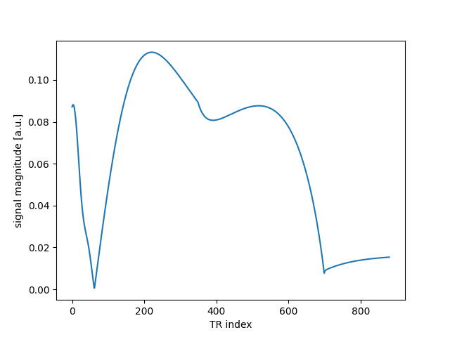
Text(33.972222222222214, 0.5, 'signal magnitude [a.u.]')

As mentioned, parallelization with automatic broadcasting is supported…

sig = mrf_sim(flip, 10.0, [1000.0, 500.0], 100.0)

plt.plot(abs(sig.T))
plt.xlabel("TR index")
plt.ylabel("signal magnitude [a.u.]")

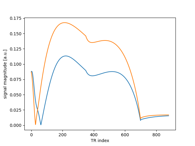
Text(25.222222222222214, 0.5, 'signal magnitude [a.u.]')

…as well as automatic differentiation controlled by diff argument:

sig, jac = mrf_sim(flip, 10.0, 1000.0, 100.0, diff=("T1", "T2"))

plt.plot(abs(jac.T))
plt.xlabel("TR index")
plt.ylabel("signal jacobian [a.u.]")

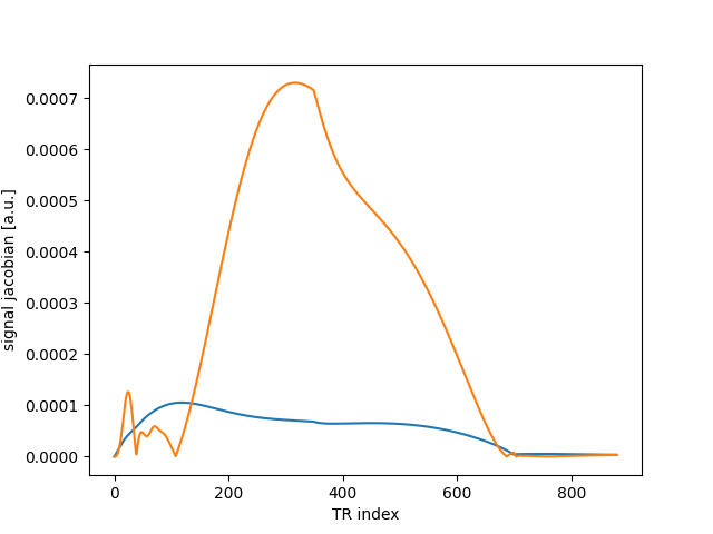
Text(16.472222222222214, 0.5, 'signal jacobian [a.u.]')