Parameter Fitting

This example shows how to use TorchSim to perform parameter inference.

We will build on the previous example. We will use numba, which can be installed as pip install numba

We’ll generate an FSE dataset from IXI database. We will neglect encoding and assume single coil for this case.

import warnings

warnings.filterwarnings("ignore")

import os
import numpy as np
import torchio as tio
import torchsim

path = os.path.realpath("data")
ixi_dataset = tio.datasets.IXI(
    path,
    modalities=("PD", "T2"),
    download=False,
)

# get subject 0
sample_subject = ixi_dataset[0]

M0 = sample_subject.PD.numpy().astype(np.float32).squeeze()[:, :, 60].T
T2w = sample_subject.T2.numpy().astype(np.float32).squeeze()[:, :, 60].T

sa = np.sin(np.deg2rad(8.0))
ta = np.tan(np.deg2rad(8.0))

T2 = -92.0 / np.log(T2w / M0)
T2 = np.nan_to_num(T2, neginf=0.0, posinf=0.0)
T2 = np.clip(T2, a_min=0.0, a_max=np.inf)

M0 = np.flip(M0)
T2 = np.flip(T2)


def simulate(T2, flip, ESP, device="cpu"):
    # get ishape
    ishape = T2.shape
    output = torchsim.fse_sim(
        flip=flip, ESP=ESP, T1=1000.0, T2=T2.flatten(), device=device
    )

    return abs(output.T.reshape(-1, *ishape)).numpy(force=True)

now generate the data

flip = 180.0 * np.ones(32, dtype=np.float32)
ESP = 5.0
device = "cpu"

# simulate acquisition
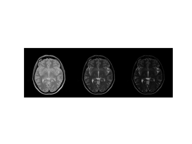
echo_series = M0 * simulate(T2, flip.copy(), ESP, device=device)

# display
img = np.concatenate((echo_series[0], echo_series[16], echo_series[-1]), axis=1)

import matplotlib.pyplot as plt

plt.imshow(abs(img), cmap="gray"), plt.axis("image"), plt.axis("off")

(<matplotlib.image.AxesImage object at 0x7ff48dfcead0>, (-0.5, 767.5, 255.5, -0.5), (-0.5, 767.5, 255.5, -0.5))

now, we want to implement a simple dictionary based inference algorithm. We first need a container to store the dictionary. We’ll use Python dataclasses for this:

from dataclasses import dataclass


@dataclass
class BlochDictionary:
    atoms: np.ndarray
    lookup_table: np.ndarray
    labels: list

    def __post_init__(self):
        self.atoms = np.ascontiguousarray(self.atoms.transpose())
        self.norm = np.linalg.norm(self.atoms, axis=0)
        self.atoms = self.atoms / self.norm
        self.lookup_table = np.ascontiguousarray(self.lookup_table.transpose())
        self.labels = list(self.labels)

    def to(self, device):
        self.atoms = self.atoms.to(device)
        self.norm = self.norm.to(device)
        self.lookup_table = self.lookup_table.to(device)
        return self

Now, we implement a simple exhaustive search algorithm. We’ll use Numba to parallelize it across different voxels:

import numba as nb

This is the main algorithm. We select matching entry using dot product as a cost function:

def _matching(signals, atoms, labels):
    """
    performs pattern matching step.
    """
    # preallocate
    cost = np.zeros(signals.shape[0], dtype=np.complex64)
    idx = np.zeros(signals.shape[0], dtype=int)

    # do actual matching
    _dot_search(signals, atoms, cost, idx)

    return labels[:, idx], cost, idx

We need to implement the dot search:

@nb.njit(fastmath=True, parallel=True)  # pragma: no cover
def _dot_search(time_series, dictionary, cost, idx):
    for n in nb.prange(time_series.shape[0]):
        for a in range(dictionary.shape[0]):
            value = _dot_product(time_series[n], dictionary[a])

            # keep maximum value
            if np.abs(value) > np.abs(cost[n]):
                cost[n] = value
                idx[n] = a

Here, we implement a trivial dot product, compatible with numba:

@nb.njit(fastmath=True, cache=True)  # pragma: no cover
def _dot_product(x, y):
    z = 0.0
    for n in range(x.shape[0]):
        z += x[n] * y[n]

    return z

We now create a wrapper to handle arbitrarily shaped inputs:

def matching(bloch_dict, time_series):
    shape = time_series.shape[1:]
    time_series = time_series.reshape((time_series.shape[0], np.prod(shape)))
    time_series = np.ascontiguousarray(time_series.transpose().conj())

    # get atoms
    atoms = np.ascontiguousarray(bloch_dict.atoms.transpose())
    labels = bloch_dict.lookup_table

    # get quantitative maps and proton density
    qmaps, cost, idx = _matching(time_series, atoms, labels)
    qmaps = qmaps.reshape([qmaps.shape[0]] + list(shape))
    qmaps = [qmap for qmap in qmaps]
    m0 = (cost / bloch_dict.norm[idx]).reshape(shape)

    return m0, dict(zip(bloch_dict.labels, qmaps))

We can assume the above code to be in a library. We now want to integrate it with our signal model from epg-torch-x. This can be done as:

import torch


def fse_fit(input, t2grid, flip, ESP, phases=None):
    if isinstance(input, torch.Tensor):
        istorch = True
        device = input.device
        input = input.numpy(force=True)
    else:
        istorch = False

    # default
    if phases is None:
        phases = -np.ones_like(flip) * 90.0

    # first build grid
    t2lut = np.linspace(t2grid[0], t2grid[1], t2grid[2])
    t1 = 1000.0

    # build dictionary
    atoms = torchsim.fse_sim(flip=flip, phases=phases, ESP=ESP, T1=t1, T2=t2lut).numpy(
        force=True
    )
    blochdict = BlochDictionary(abs(atoms), t2lut[:, None], ["T2"])

    # perform matching
    m0, maps = matching(blochdict, input)

    # here, we only have T2
    t2map = maps["T2"]

    # cast back
    if istorch:
        m0 = torch.as_tensor(m0, device=device)
        t2map = torch.as_tensor(t2map, device=device)

    return m0, t2map

Done! We can now try it:

M0rec, T2rec = fse_fit(echo_series.copy(), (1.0, 350.0, 1000), flip.copy(), ESP)

plt.subplot(2, 2, 1)
plt.imshow(T2, vmax=350.0), plt.axis("off"), plt.colorbar(), plt.title("true T2 [ms]")
plt.subplot(2, 2, 2)
plt.imshow(T2rec, vmax=350.0), plt.axis("off"), plt.colorbar(), plt.title(
    "recon T2 [ms]"
)
plt.subplot(2, 2, 3)
plt.imshow(M0, cmap="gray"), plt.axis("off"), plt.colorbar(), plt.title("true M0")
plt.subplot(2, 2, 4)
plt.imshow(abs(M0rec), cmap="gray"), plt.axis("off"), plt.colorbar(), plt.title(
    "recon M0"
)

(<matplotlib.image.AxesImage object at 0x7ff48cc0cac0>, (-0.5, 255.5, 255.5, -0.5), <matplotlib.colorbar.Colorbar object at 0x7ff48cc0f490>, Text(0.5, 1.0, 'recon M0'))