Synthetic Data Generation

This example shows how to use TorchSim to generate synthetic data.

We will use torchio and sigpy to get realistic ground truth maps and coil sensitivities. These can be installed as:

pip install torchio pip install sigpy

We will use realistic maps from the IXI dataset, downloaded using torchio:

import warnings

warnings.filterwarnings("ignore")

import os
import torchio as tio

path = os.path.realpath("data")
ixi_dataset = tio.datasets.IXI(
    path,
    modalities=("PD", "T2"),
    download=False,
)

# get subject 0
sample_subject = ixi_dataset[0]

We will now extract an example slice and compute M0 and T2 maps to be used as simulation inputs.

import numpy as np

M0 = sample_subject.PD.numpy().astype(np.float32).squeeze()[:, :, 60].T
T2w = sample_subject.T2.numpy().astype(np.float32).squeeze()[:, :, 60].T

Compute T2 map:

sa = np.sin(np.deg2rad(8.0))
ta = np.tan(np.deg2rad(8.0))

T2 = -92.0 / np.log(T2w / M0)
T2 = np.nan_to_num(T2, neginf=0.0, posinf=0.0)
T2 = np.clip(T2, a_min=0.0, a_max=np.inf)

M0 = np.flip(M0)
T2 = np.flip(T2)

Now, we can create our simulation function

Let’s use torchsim fse simulator

import torchsim


def simulate(T2, flip, ESP, device="cpu"):
    # get ishape
    ishape = T2.shape
    output = torchsim.fse_sim(
        flip=flip, ESP=ESP, T1=1000.0, T2=T2.flatten(), device=device
    )

    return output.T.reshape(-1, *ishape).numpy(force=True)

Assume a constant refocusing train

flip = 180.0 * np.ones(32, dtype=np.float32)
ESP = 5.0
device = "cpu"

# simulate acquisition
echo_series = M0 * simulate(T2, flip, ESP, device=device)

# display
img = np.concatenate((echo_series[0], echo_series[16], echo_series[-1]), axis=1)

import matplotlib.pyplot as plt

plt.imshow(abs(img), cmap="gray"), plt.axis("image"), plt.axis("off")

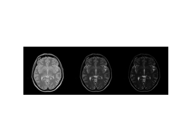
(<matplotlib.image.AxesImage object at 0x7ff497956920>, (-0.5, 767.5, 255.5, -0.5), (-0.5, 767.5, 255.5, -0.5))

Now, we want to add coil sensitivities. We will use Sigpy:

import sigpy.mri as smri

smaps = smri.birdcage_maps((8, *echo_series.shape[1:]))

We can simulate effects of coil by simple multiplication:

echo_series = smaps[:, None, ...] * echo_series
print(echo_series.shape)

(8, 32, 256, 256)

Now, we want to simulate k-space encoding. We will use a simple Poisson Cartesian encoding from Sigpy.

import sigpy as sp

mask = np.stack([smri.poisson(T2.shape, 32) for n in range(32)], axis=0)
ksp = mask * sp.fft(echo_series, axes=range(-2, 0))

plt.imshow(abs(ksp[0, 0]), vmax=50), plt.axis("image"), plt.axis("off"), plt.colorbar()

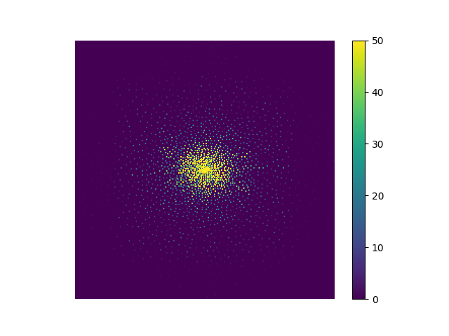
(<matplotlib.image.AxesImage object at 0x7ff49449a110>, (-0.5, 255.5, 255.5, -0.5), (-0.5, 255.5, 255.5, -0.5), <matplotlib.colorbar.Colorbar object at 0x7ff494143a90>)

Potentially, we could use Non-Cartesian sampling and include non-idealities such as B0 accrual and T2* decay during readout using mri-nufft.

Now, we can wrap it up:

def generate_synth_data(M0, T2, flip, ESP, phases=None, ncoils=8, device="cpu"):
    echo_series = M0 * simulate(T2, flip, ESP, device=device)
    smaps = smri.birdcage_maps((ncoils, *echo_series.shape[1:]))
    echo_series = smaps[:, None, ...] * echo_series
    mask = np.stack(
        [smri.poisson(T2.shape, len(flip)) for n in range(len(flip))], axis=0
    )
    return mask * sp.fft(echo_series, axes=range(-2, 0))

Reconstruction shows the effect of undersampling:

ksp = generate_synth_data(M0, T2, flip, ESP, device=device)
recon = sp.ifft(ksp, axes=range(-2, 0))
recon = (recon**2).sum(axis=0) ** 0.5
img = np.concatenate((recon[0], recon[16], recon[-1]), axis=1)
plt.imshow(abs(img), cmap="gray"), plt.axis("image"), plt.axis("off")

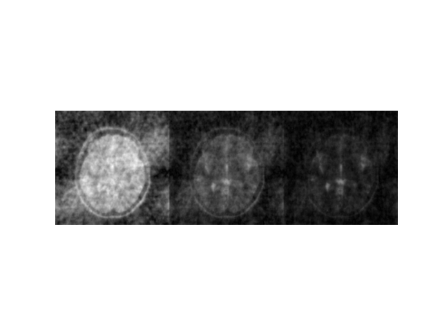
(<matplotlib.image.AxesImage object at 0x7ff48dfae440>, (-0.5, 767.5, 255.5, -0.5), (-0.5, 767.5, 255.5, -0.5))

This can be combined with data augmentation in torchio to generate synthetic datasets, such as in Synth-MOLED.